Understanding Orbital Uncertainties in the Context of Impact Predictions
II: Orbit Fitting-Least Squares Technique for Orbit Estimation
This is the second in a series of articles detailing the concept of orbital uncertainties as it relates to impact predictions. Celestial mechanics can be a complicated subject, but here we'll try to distill some of these difficulties and render the subject a bit more transparent.
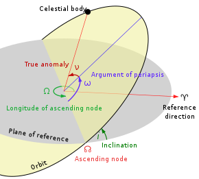
Orbital elements
Credit: (Lasunncty at the English Wikipedia, CC BY-SA 3.0, via Wikimedia Commons
Our previous article described some of the quantities required for determining an orbit, and thus for predicting where objects will be at any point in the future. We discussed the need for 6 orbital elements and presented 3: eccentricity, inclination, and semi-major axis. The remaining 3 involve the orientation of the ellipse and the time when the object is at its closest point to the sun.
In practice we never really measure these orbital elements-rather we measure positions in space and time, and when we measure enough of these we can compute the full orbit. The actual mathematics is a little complicated and really beyond what we need to discuss here, but the point is that solutions exist for these problems and the calculations are routine on modern computers. All of these calculations rely on the concept of least squares, a mathematical technique that computes the best fit to a set of points. The least squares method was first published by Legendre in 1805, but Gauss had used a form of it for the orbital solution for the first minor planet Ceres , found in 1801.
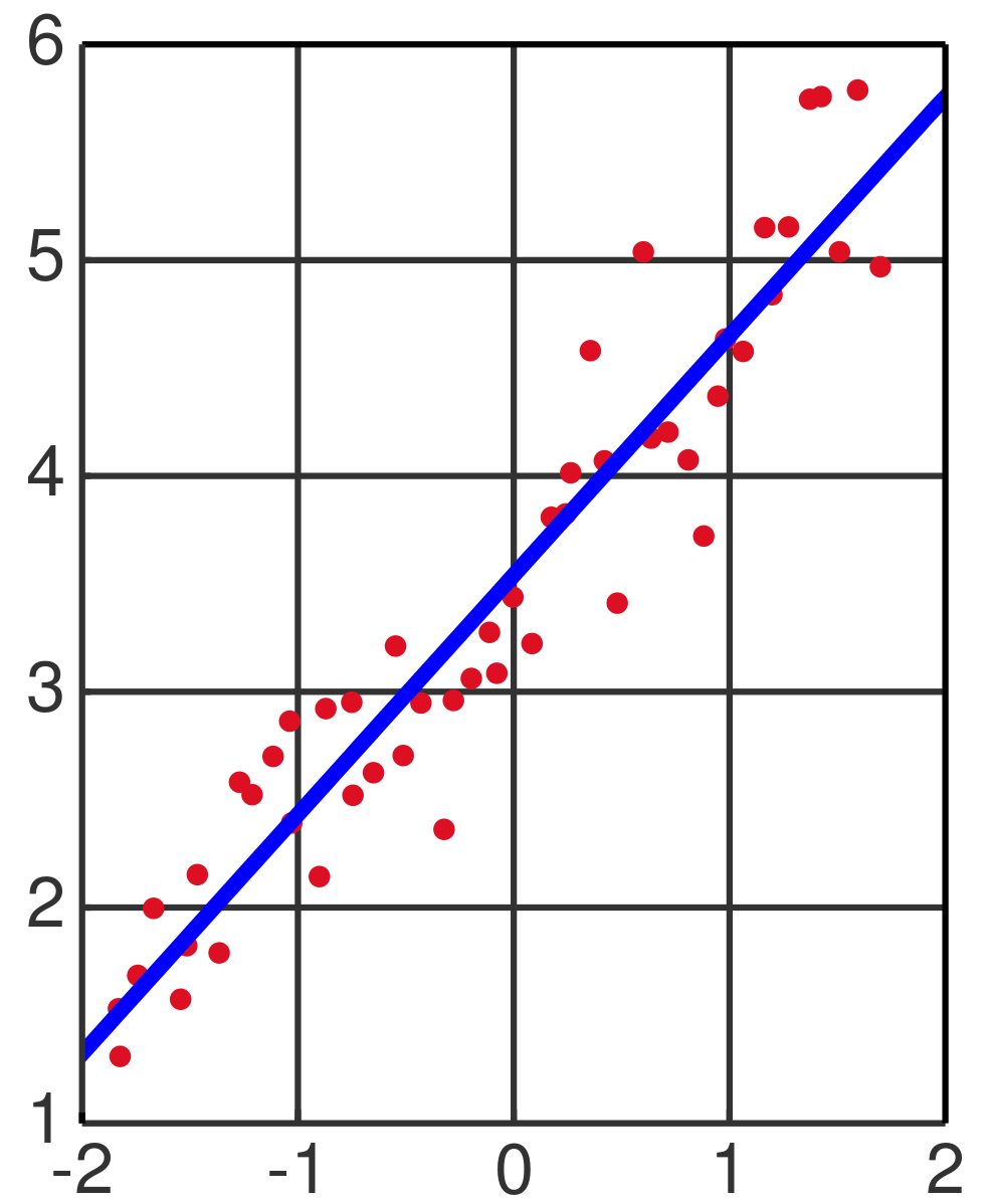
Illustration of linear least squares.
Credit: (Oleg Alexandrov at the English Wikipedia via Wikimedia Commons
The least squares method works best when we have sets of constraints on our mathematical problem. For example, if you know you have an equation that represents a line in an X-Y graph, then you can assume that particular form for the solution.
For orbital elements, our assumption is that the orbits are elliptical and this reduces the complexity of the least squares solution dramatically. Note that even if the orbit is hyperbolic, this is still a conic section and the math is quite similar to the elliptical calculations and one can use the same methods. This means it was just as easy to compute the orbit for 2I/Borisov on a strongly hyperbolic orbit as it was to compute the orbit for 175P/Hergenrother, a short-period comet that orbits the sun every ~7 years.
In the next article in this series, we will discuss 'astrometry', or the measurement of positions and times using astronomical coordinate systems. Accurate and precise astrometry is the currency by which all orbits are effectively computed.